Blogs

Shading Rows with Conditional Formatting

If you haven't tried out the conditional formatting features of Excel before, they can be quite handy. One way to use this feature is to cause Excel to shade every other row in your data. This is great when your data uses a lot of columns and you want to make it a bit easier to read on printouts. (this is different from the “Design” layout). Simply follow these steps:
 

1. Select the data whose alternating rows you want to shade.
2. Make sure the Home tab of the ribbon is displayed.
3. Click the Conditional Formatting tool. Excel displays a series of choices.
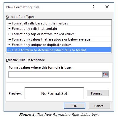
4. Click New Rule. Excel displays the New Formatting Rule dialog box.
5. In the Select a Rule Type area at the top of the dialog box, choose Use a Formula to Determine Which Cells to Format. (See Figure 1.)
    

6. In the formula space, enter the following formula: =MOD(ROW(),2)=0
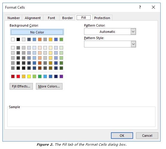
7. Click on the Format button. Excel displays the Format Cells dialog box.
8. Make sure the Fill tab is selected. (See Figure 2.)
     

9. Select the color you want used for the row shading.
10. Click on OK to close the Format Cells dialog box.
11. Click on OK to close the New Formatting Rule dialog box.